Real-time data warehouse introductory training camp: real-time calculation of Flink version SQL practice

Introduction to "Real-time Data Warehouse Introductory Training Camp" consists of Alibaba Cloud researcher Wang Feng, Alibaba Cloud senior product expert Liu Yiming and other real-time computing Flink version and Hologres technology/product front-line experts joined the battle to build the training camp course. System, carefully polished the content of the course, and directly hit the pain points encountered by the current students. Analyze the architecture, scenarios, and practical applications of real-time data warehouses from the shallower to the deeper, and 7 high-quality courses will help you grow from a small white to a big cow in 5 days!

This article is compiled from the live broadcast "Real-time Computing Flink Edition SQL Practice-Li Lin (Sea Leopard)"
Video link: https://developer.aliyun.com/learning/course/807/detail/13887

Brief content:
1. Introduction to real-time computing Flink version SQL
Two, real-time calculation of Flink version SQL hands-on example
3. Develop common problems and solutions

Introduction to real-time calculation of Flink version of SQL

(1) About real-time calculation of Flink version SQL

The real-time computing Flink version chose SQL as the top-level API, which is relatively stable and user-friendly. Flink SQL has the characteristics of unified flow and batch, giving users a unified development experience and consistent semantics. In addition, Flink SQL can automatically optimize, including shielding the complexity of the State in the flow calculation, and also provides an automatically optimized Plan, and also integrates the AutoPilot automatic tuning function. Flink SQL has a wide range of application scenarios, including data integration, real-time reporting, real-time risk control, and online machine learning.

(2) Basic operation

In the basic operation, you can see that the syntax of SQL is very similar to standard SQL. The example includes basic SELECT and FILTER operations. , You can use built-in functions, such as date formatting, or you can use custom functions. For example, the exchange rate conversion in the example is a user-defined function, which can be used directly after registration on the platform.

(3) Dimensional table Lookup Join

In the actual data processing process, the Lookup Join of the dimension table is also a relatively common example.

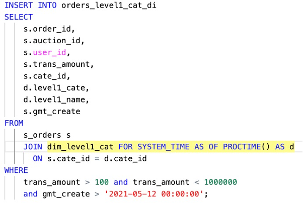
Shown here is an example of a dimension table INNER JOIN.

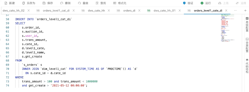
The SOURCE table shown in the example is a real-time change order information table. It uses INNER JOIN to associate dimension table information. Here, the grammar of dimension table JOIN is highlighted in yellow. You can see that it is written in the same way as traditional batch processing. The difference is that the clause FOR SYSTEM\_TIME AS OF is added to indicate that it is a JOIN operation of a dimension table. Every time an order message comes from the SOURCE table, it will trigger the dimension table operator to do a query on the dimension table information, so it is called a Lookup Join.

(4) Window Aggregation

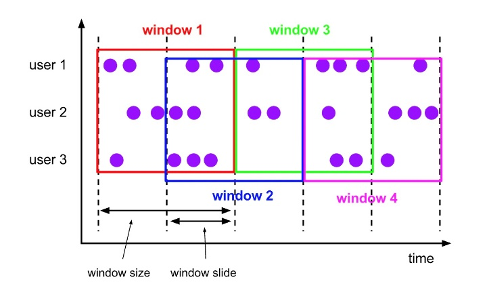
Window Aggregation (window aggregation) operations are also common operations. Flink SQL has built-in support for several commonly used Window types, such as Tumble Window, Session Window, Hop Window, and the newly introduced Cumulate Window.

Tumble

Tumble Window can be understood as a fixed-size time window, also called a rolling window, such as a window with a fixed interval of 5 minutes, 10 minutes, or 1 hour, and there is no overlap between the windows.

Session

Session Window (session window) defines the scope of a continuous event, a parameter in the window definition is called Session Gap, which means that if the interval between two pieces of data exceeds the defined duration, the previous Window will end and a new one will be generated at the same time window.

Hop

Hop Window is different from the rolling window. The windows of the sliding window can overlap. The sliding window has two parameters: size and slide. size is the size of the window, and slide is the step length of each sliding. If slide <size, the windows will overlap and the same piece of data may be allocated to multiple windows; if slide = size, it is equivalent to Tumble Window. If slide> size, there is no overlap and gaps between the windows.

Cumulate

Cumulate Window (cumulative window) is newly introduced in version 1.13 of Flink community. It can be understood by comparing Hop Window. The difference is that it continues to accumulate from Window Start. In the example, Window 1, Window 2, and Window 3 are constantly growing. It has a maximum window length. For example, if we define Window Size to be one day, and Step step size is 1 hour, then it will produce aggregate results accumulated to the current hour in each hour of the day.

Look at a specific window aggregation processing example.

As shown in the figure above, for example, it is necessary to count the number of clicks of a single user every 5 minutes.

The source data is the user's click log. We expect to calculate the total number of clicks by a single user every 5 minutes. The SQL uses the community's latest WindowTVF syntax. First open the source table, and then the attributes window\_start and window corresponding to the GROUP BY window \_end, COUNT(*) is the click count.

It can be seen that when processing the data from 12:00 to 12:04, 2 users have generated 4 clicks. It can be counted that the user Mary is 3 times and Bob is 1 time. In the next batch of data, there are three more data, which are updated to the next window correspondingly, 1 time and 2 times respectively.

(5) Group Aggregation

Compared with Window Aggregation, Group Aggregation directly triggers the calculation, and does not need to wait until the end of the window. One applicable scenario is to calculate the cumulative value.

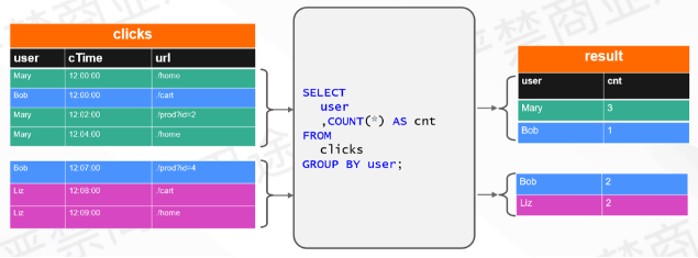
The example above is the statistics of the number of clicks accumulated by a single user to the current time. From the Query point of view, the writing method is relatively simple, just use GROUP BY user to calculate COUNT(*), which is the cumulative count.

It can be seen that there is a difference between the results and the output of Window. In the first 4 input data that are the same as Window, the output result of Group Aggregation is that Mary’s clicks have been updated to 3 times. The specific calculation process may be from 1 becomes 2 and then becomes 3, Bob is once, with the input of the following 3 pieces of data, the number of clicks corresponding to Bob will be updated to 2 again, and the result is a continuous update process, which is the same as the calculation scenario of Window There are some differences.

The data output in the previous Window window will not change the result after the window ends. In Group Aggregation, the result of the same Group Key will be continuously updated.

(6) Window Aggregation Vs Group Aggregation

A more comprehensive comparison of some of the differences between Window and Group Aggregation.

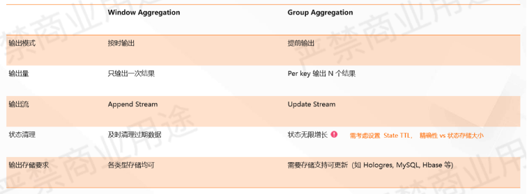
Window Aggregation is output on time in the output mode, and it will output only after the defined data expires. For example, if you define a 5-minute window, the result is output delayed. For example, for the time period of 00:00~00:05, it will wait for the data in the entire window to arrive before the complete output, and the result will only be output once, not again Change.

Group Aggregation is a data trigger. For example, the first piece of data will output the result, and the second piece of data of the same key will update the result, so the nature of the output stream is different. Window Aggregation generally outputs Append Stream, while in Group Aggregation, it outputs Update Stream.

The difference between the two in state processing is also relatively large. Window Aggregation will automatically clean up expired data, so users don't need to pay attention to the expansion of State. Group Aggregation is based on an infinite state to do accumulation, so users need to define the TTL of the State according to their own calculation scenarios, which is how long the State is stored.

For example, count the PV and UV accumulated in a day, regardless of the data delay, and at least ensure that the TTL of the State is greater than or equal to one day, so as to ensure the accuracy of the calculation. If the TTL of State is defined as half a day, the statistical value may be inaccurate.

The storage requirements for the output are also determined by the nature of the output stream. On Window's output, because it is an Append stream, all types can be docked and output. The Group Aggregatio outputs the update stream, so the target storage is required to support updates. You can use Hologres, MySQL, or HBase, which support updates.

Real-time calculation of Flink version SQL hands-on example

Let's see how each SQL operation is used in real business scenarios through specific examples, such as basic SQL syntax operations, including the use of some common aggregations.

(1) Example scenario description: e-commerce transaction data-real-time data warehouse scenario

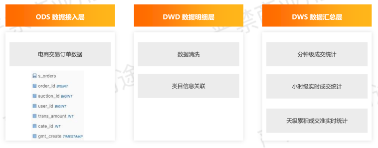
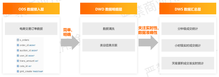
The example here is an e-commerce transaction data scenario, which simulates the situation of hierarchical data processing in a real-time data warehouse.

In the data access layer, we simulate the transaction order data of the e-commerce, which includes basic information such as order ID, product ID, user ID, transaction amount, product leaf category, transaction time, etc. This is a simplified table.

Example 1 will complete a data cleaning work from the access layer to the data detail layer. In addition, it will also associate category information. Then, at the data aggregation layer, we will demonstrate how to complete minute-level transaction statistics and how to do real-time hourly level statistics. Transaction statistics. Finally, I will introduce how to do quasi-real-time statistics on the transaction scenarios accumulated at the sky level.

-Example environment: internal beta version

The demonstration environment is a real-time computing Flink product in the current internal beta version. On this platform, you can directly do one-stop job development, including debugging, as well as online operation and maintenance.

-Access layer data

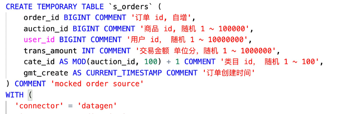
Use SQL DataGen Connector to generate simulated e-commerce transaction data.

Access layer data: In order to facilitate demonstration and simplify the link, use the built-in SQL DataGen Connector to simulate the generation of e-commerce data.

Here, order\_id is designed with an auto-increment sequence, and the parameters of the Connector are not completely posted. DataGen Connector supports several generation modes. For example, Sequence can be used to generate self-incrementing sequences, and Random mode can simulate random values. Here, according to the business meaning of different fields, different generation strategies are selected.

For example, order\_id is self-increasing, the product ID is randomly selected from 10,000 to 100,000, and the user ID is from 10,000 to 10 million. The transaction amount is used as the unit. cate\_id is the leaf category ID. Here, a total of 100 leaves are simulated. The category is generated directly by taking the remainder of the product ID through the calculation column, and the order creation time is simulated using the current time, so that it can be debugged on the development platform without the need to create Kafka or DataHub to simulate the access layer.

(2) Example 1-1 Data cleaning

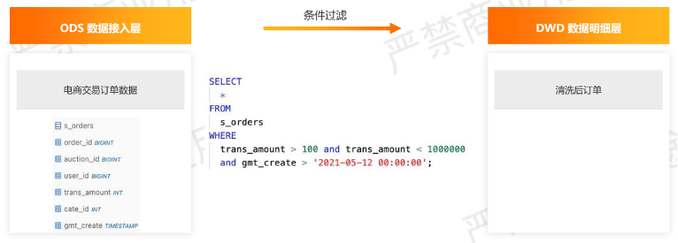
-e-commerce transaction data-order filtering

This is a data cleaning scenario. For example, when order filtering needs to be completed on the business, the business party may filter the maximum and minimum abnormalities of the transaction amount. For example, it must be greater than 1 yuan and less than 10,000 to retain valid data.

The creation time of the transaction is selected after a certain moment, and this logic can be completed by filtering through the combination of WHERE conditions.

The real business scenario may be a lot more complicated, let's take a look at how SQL runs.

This is using the debugging mode. Click the Run button on the platform to perform local debugging. You can see that the column of amount is filtered, and the order creation time is also greater than the required time value.

From this simple cleaning scenario, it can be seen that compared with traditional batch processing in real-time, there is not much difference in writing including output results. The main difference between stream jobs is that they keep running for a long period of time after running, unlike traditional batch processing. Batch processing ends after processing the data.

(3) Example 1-2 Association of category information

Next, let's take a look at how to do dimension table association.

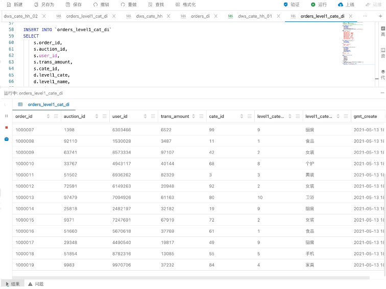
According to the order data of the access layer just now, because the original data contains the leaf category information, the dimension table of the associated category is required in the business. The dimension table records the association relationship, ID and name of the leaf category to the first-level category. , The goal to be completed in the cleaning process is to associate the dimension table with the leaf category ID in the original table, and complement the ID and Name of the first-level category. Here, the INNER JOIN dimension table is written, and the fields corresponding to the dimension table are selected after association.

The difference between the writing method and the batch processing is only in the special syntax FOR SYSTEM\_TIME AS OF of the dimension table.

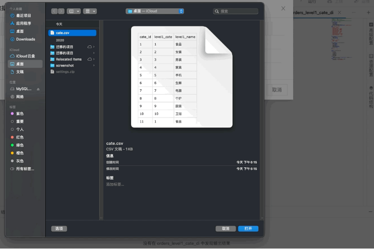
As shown above, you can upload your own data for debugging on the platform. For example, 1 CSV test data is used here, and 100 leaf categories are mapped to 10 first-level categories.

The single digit of the corresponding leaf category ID is its first-level category ID, which will be associated with the corresponding first-level category information, and its name will be returned. The advantage of local debugging operation is that the speed is relatively fast, and the results can be seen immediately. In the local debugging mode, after the terminal receives 1000 pieces of data, it will automatically pause to prevent the result from being too large and affecting the use.

(4) Example 2-1 minute-level transaction statistics

Next we look at the statistics based on Window.

The first scenario is the minute-level transaction statistics, which is a commonly used calculation logic in the summary layer.

It is easy to think of Tumble Window for minute-level statistics. Every minute is counted separately. Several indicators need to be calculated, including the total number of orders, the total amount, the number of goods traded, and the number of users who traded. The number of items traded and the number of users need to be de-duplicated, so a Distinct is made in the writing.
The window is the Tumble Window just introduced. It draws a one-minute window according to the order creation time, and then counts the transaction status of each minute according to the dimensions of the first category.

-Operating mode

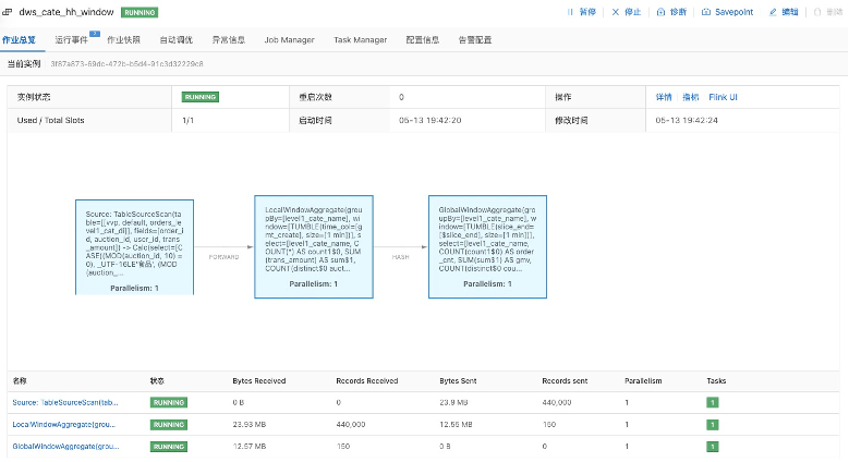
The above picture is a bit different from the debugging mode just now. After going online, it is actually submitted to the cluster to run a job, and its output uses the debugging output, which is printed directly to the Log. Expand the job topology and you can see that the two-stage optimization of Local-Global is automatically turned on.

-Run log-View debugging output

After running for a period of time, you can see the final output result through the log in the Task.

The print sink is used, and it will be directly printed into the log. In the output of real scenes, such as writing to Hologres/MySQL, you need to check the corresponding storage database.

It can be seen that the output data has a certain lag relative to the original time of the data.

At 19:46:05, the data of the 19:45:00 window was output, and the aggregation results of the previous 1 minute were output after a delay of about 5 seconds.

These 5 seconds are actually related to the setting of WATERMARK when the source table is defined. When the WATERMARK is declared, the offset of 5 seconds is added to the gmt\_create field. The effect of this is that when the earliest data that arrives is 19:46:00, we think that the water mark is 19:45:55, which is the 5 second delay effect to achieve tolerance processing of out-of-order data.

(5) Example 2-2 hour-level real-time transaction statistics

The second example is to do hourly real-time transaction statistics.

As shown in the figure above, when real-time statistics are required, open the Tumble Window directly into a Tumble Window of 1 hour size. Can this satisfy real-time performance? According to the output result just shown, it has a certain delay effect. Therefore, when you open a window of one hour, you must wait until the data of this hour is received. At the beginning of the next hour, the results of the previous hour can be output. The delay is at the hour level, which cannot meet the real-time requirements. Looking back at the Group Aggregation introduced earlier, it can meet real-time requirements.

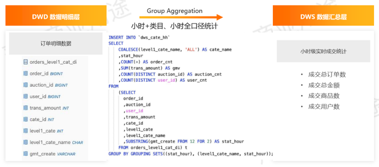
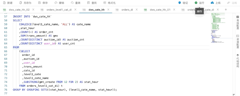
Specifically, for example, it is necessary to complete the two-caliber statistics of hour + category and hour only. The two statistics are done together. The GROUPING SETS function commonly used in traditional batch processing is also supported on real-time Flink.

We can directly GROUP BY GROUPING SETS, the first is the full-caliber of the hour, the second is the statistical caliber of category + hour, and then calculate the number of its orders, including the total amount, the number of deduplicated products and the number of users.

This way of writing adds a null value conversion process to the result for easy viewing of the data, that is, the full-caliber statistics of the hour, the output of the first-level category is empty, and a null value conversion process needs to be performed on it.

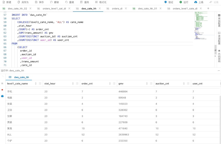
The above is the running process in debug mode. You can see that the data generated by Datagen is updated to the first level category and its corresponding hour in real time.

It can be seen here that the results of two different GROUP BYs are output together, and there is a column of ALL in the middle that is converted by a null value, which is the full-caliber statistical value. Local debugging is relatively intuitive and convenient. If you are interested, you can apply or purchase it on the official website of Alibaba Cloud to experience it.

(6) Example 2-3 day-level cumulative transaction statistics in real time

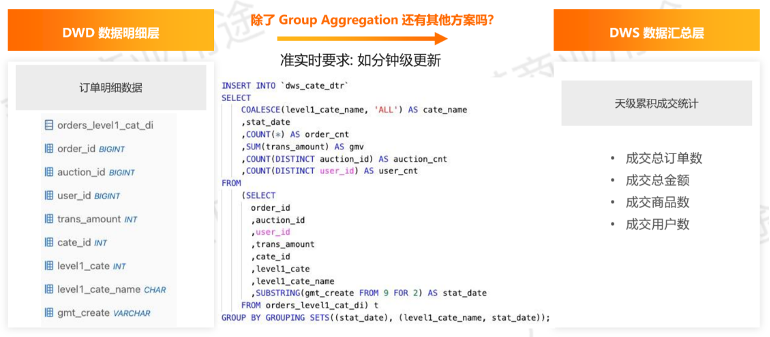
The third example is day-level accumulated transaction statistics. The business requirement is quasi-real-time, such as being able to accept minute-level update delays.

According to the real-time statistics of Group Aggregation hours just now, it is easy to think of directly changing the Query to the sky dimension to achieve this requirement, and the real-time performance is relatively high, and the data can be updated in seconds after the data is triggered.

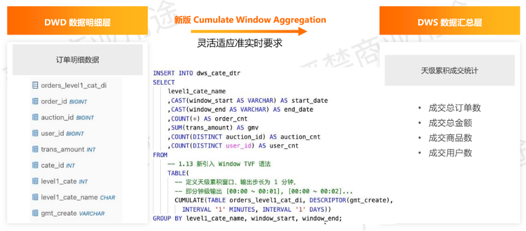
Recalling the previously mentioned difference between Window and Group Aggregation for the built-in state processing, Window Aggregation can automatically clean up the State, and Group Aggregation requires users to adjust the TTL by themselves. Since the business requires quasi-real-time, there can be an alternative solution here, such as using the newly introduced Cumulate Window to do cumulative Window calculations, day-level accumulation and then using minute-level steps, which can achieve accurate updates every minute. Real-time requirements.

Review the Cumulate Window, as shown above. If the sky level is accumulated, the maximum size of the Window is up to the day, and its Window Step is one minute, so that the accumulated statistics of the sky level can be expressed.

The specific Query is as above. Here, the new TVF syntax is used, and the definition of Windows is included in the middle through a TABLE keyword, and then Cumulate Window refers to the input table, and then defines its time attribute, step size and size parameters. GROUP BY is a common way of writing, because it has early output, so we print out the start time and end time of the window together.

This example also runs online to see the Log output.

-Operating mode

It can be seen that it is similar to the structure of the previous Tumble Window operation, and it is also pre-aggregation plus global aggregation. The difference between it and Tumble Window is that it does not need to wait until the data is available on this day to output the results.

-Run log-observe the debugging results

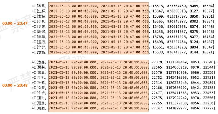
As can be seen from the example above, at 20:47:00, there are already accumulated results from 00:00:00 to 20:47:00, and there are corresponding 4 columns of statistical values. The next output is the next cumulative window. You can see that 20:47:00 to 20:48:00 is a cumulative step length, which not only meets the daily cumulative statistics requirements, but also meets the quasi-real-time requirements.

(7) Example summary: E-commerce transaction data-real-time data warehouse scenario

Then let's summarize the above example as a whole.

The cleaning process from the access layer to the detail layer is relatively simple and clear. For example, the business logic requires fixed filtering conditions, including the expansion of dimensions, which are very clear and straightforward.

From the detail level to the summary level, we used Tumble Window for the minute-level statistics in the example, and the hour-level was replaced by Group Aggregation due to real-time requirements, and then to the day-level accumulation to show Group Aggregation and the newly introduced Cumulate. Window.

From the calculation characteristics of the summary layer, we need to pay attention to the real-time requirements and data accuracy requirements of the business, and then choose Window aggregation or Group aggregation according to the actual situation.

Why is data accuracy mentioned here?

When comparing Window Aggregation and Group Aggregation at the beginning, it was mentioned that Group Aggregation has very good real-time performance, but its data accuracy depends on State TTL. When the statistical period is greater than TTL, then TTL data may be distorted.

On the contrary, in Window Aggregation, there is an upper limit on the tolerance of disorder, such as waiting at most one minute, but in actual business data, 99% of the data may meet such requirements, and 1% of the data may be It will take an hour to come. Based on the processing of WATERMARK, it is a discarding strategy by default. The data that exceeds the maximum offset will be discarded and will not be included in the statistics. At this time, the data will also lose its accuracy, so this is a relative indicator and needs to be based on Choose specific business scenarios.

Develop common problems and solutions

(1) Common problems in development

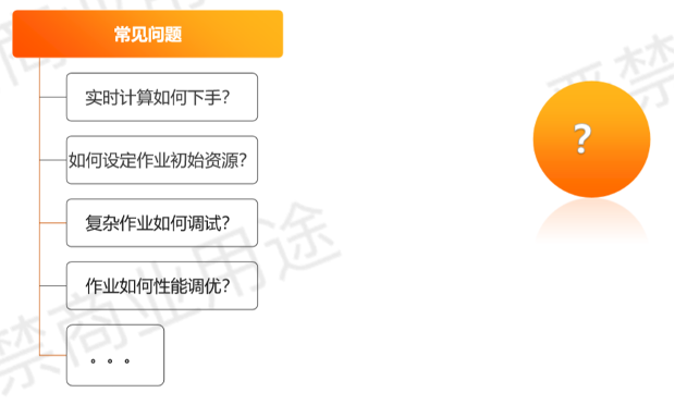
The above is a relatively high-frequency problem in the real-time calculation of real business contacts.

The first is that real-time computing does not know how to start, how to start real-time computing, for example, some students have a batch processing background, and then just started to contact Flink SQL, do not know where to start.

Another type of problem is that the SQL has been written, and it is also clear what level of data the input processing is, but I don’t know how much resources need to be set after the real-time job runs.

There is also a type of SQL that is more complicated to write, and debugging is required at this time. For example, to check why the calculated data does not meet expectations and other similar problems, many students report that they have no way to start.

How to tune the job after running is also a very high frequency problem.

(2) Develop solutions to common problems

1. How to start real-time calculation?

For the problem of getting started, the community has many official documents and some examples are provided. You can start with simple examples and slowly understand the different operators in SQL and what kind of characteristics they will have in stream computing.

In addition, you can also follow the developer community's real-time calculation of Flink version, ververica.cn website, Apache Flink official account of station B and other shared content.

After getting familiar with SQL, if you want to apply it to the production environment to solve real business problems, Alibaba Cloud's industry solutions also provide some typical architecture designs, which can be used as references.

2. How to debug complex operations?

If you encounter thousands of lines of complex SQL, even for Flink development students, you cannot locate the problem at a glance. In fact, you still need to follow the process from simple to complex, and you may need to use some debugging tools, such as the platform demonstrated above. Debug function, and then perform segmented verification. After debugging the correctness of the partial SQL results, they are assembled step by step to finally make this complex operation meet the correctness requirements.

In addition, you can use the features of SQL syntax to organize SQL more clearly. There is a code structure function on real-time calculation Flink products, which can easily locate specific statements in long SQL. These are some auxiliary tools.

3. How to tune the initial resource settings of the job?

One experience we have is to initially do a small concurrency test based on the input data to see how it performs, and then estimate it. In large-concurrent stress testing, gradually approaching according to the required throughput, and then getting the expected performance configuration, this is a relatively straightforward but relatively reliable way.

The tuning part is mainly based on the operation of the job. We will pay attention to some key indicators, such as whether there is data skew, the Lookup Join of the dimension table needs to access external storage, and whether there is an IO bottleneck. It is a common bottleneck that affects job performance and requires attention.

A function called AutoPilot is integrated in the real-time computing Flink product, which can be understood as similar to automatic driving. Under this function, the initial resource setting is not a troublesome question.

On the product, after setting the maximum resource limit for the job, according to the actual data processing volume, how much resources should be used can be automatically adjusted to the optimal state by the engine and scaled according to the load situation.

Copyright Statement: content of this article is contributed spontaneously by Alibaba Cloud real-name registered users, and the copyright belongs to the original author. The Alibaba Cloud Developer Community does not own its copyright and does not assume corresponding legal responsibilities. For specific rules, please refer to the "Alibaba Cloud Developer Community User Service Agreement" and the "Alibaba Cloud Developer Community Intellectual Property Protection Guidelines". If you find suspected plagiarism in this community, fill in the infringement complaint form to report it. Once verified, the community will immediately delete the suspected infringing content.