Classifying color flower images - Keras implementation based on R language

This case is excerpted from the comprehensive case content in Chapter 4 of "Keras Deep Learning Introduction, Practice and Advancement". The data for this case comes from Flower Color on Kaggle.

Researcher at Microsoft MVP Labs

The data content is very simple: contains 210 images (128×128×3) of 10 flowering plants and the file flower-labels.csv with labels, the photo files are in .png format, and the labels are integers (0~9). Import the file flower-labels.csv with labels into R using read.csv() and look at the first six rows.

 > flowers <- read.csv('../flower_images/flower_labels.csv')
> dim(flowers)
[1] 210   2
> head(flowers)
      file label
1 0001.png     0
2 0002.png     0
3 0003.png     2
4 0004.png     0
5 0005.png     0
6 0006.png     1

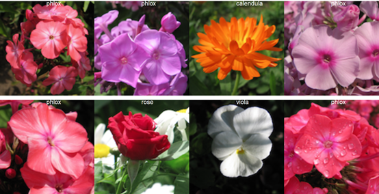
There are a total of 210 rows and 2 columns, the first column is the image file name, and the second column is its corresponding label value. The color images numbered 0001, 0002, 0004, and 0005 have the corresponding label of 0, which is phlox; the 0003 color image has a label of 2, which is calendula; the 0006 color image has a label of 1, which is Rose.
label is the target variable, use the as.matrix() function to convert it into a matrix, and then use the to_categorical() function to convert it to one-hot encoding. The converted data is as follows.

 > flower_targets <- as.matrix(flowers["label"])
> flower_targets <- keras::to_categorical(flower_targets, 10)
> head(flower_targets)
      [,1]   [,2]  [,3]  [,4]   [,5]  [,6]  [,7]  [,8]  [,9]  [,10]
[1,]    1    0    0    0    0    0    0    0    0     0
[2,]    1    0    0    0    0    0    0    0    0     0
[3,]    0    0    1    0    0    0    0    0    0     0
[4,]    1    0    0    0    0    0    0    0    0     0
[5,]    1    0    0    0    0    0    0    0    0     0
[6,]    0    1    0    0    0    0    0    0    0     0

The file names of all color images in the flower_images directory can be obtained using the list.files() function.

 > # 获取flower_images目录中的彩色照片
> image_paths <- list.files('../flower_images',pattern = '.png')
> length(image_paths)
[1] 210
> image_paths[1:3]
[1] "0001.png" "0002.png" "0003.png"

There are a total of 210 color images in the flower_images directory. The names of the first 3 image files are "0001.png", "0002.png", and "0003.png". Use the readImage() function of the EBImage package to read the first 8 colored images into R and visualize them.

 > names <- c('phlox','rose','calendula','iris',
+             'max chrysanthemum','bellflower','viola',
+             'rudbeckia laciniata','peony','aquilegia')
> options(repr.plot.width=4,repr.plot.height=4)
> op <- par(mfrow=c(2,4),mar=c(2,2,2,2))
> for(i in 1:8){
+   img <- readImage(paste('../flower_images',image_paths[i],sep = '/')) # 读入图像
+   plot(img)                                                # 绘制图像
+   text(x = 64,y = 0,
+        label = names[flowers[flowers$file==image_paths[i],'label']+1],
+        adj = c(0,1),col = 'white',cex = 3)                         # 添加标签
+ }
> par(op)

Customize the image_loading() function to gradually read the color image of flower_iamges into R, and perform data conversion to make it meet the independent variable matrix required for deep learning modeling.

 > # 自定义图像数据读入及转换函数
> image_loading <- function(image_path) {
+   image <- image_load(image_path, target_size=c(128,128))
+   image <- image_to_array(image) / 255
+   image <- array_reshape(image, c(1, dim(image)))
+   return(image)
+ }

Combined with the lapply() function to read 210 flower color images in the flower_images directory, since the returned result is a list, the array_reshape() function is used to convert it again.

 > image_paths <- list.files('../flower_images',
+                    pattern = '.png',
+                    full.names = TRUE)
> flower_tensors <- lapply(image_paths, image_loading)
> flower_tensors <- array_reshape(flower_tensors,
+                           c(length(flower_tensors),128,128,3))
> dim(flower_tensors)
[1] 210 128 128   3
> dim(flower_targets)
[1] 210  10

We use the createDataParitition() function of the caret package to sample the data in equal proportions, so that the proportion of each category in the training set and test set after sampling is the same as the original data.

 > # 等比例抽样
> index <- caret::createDataPartition(flowers$label,p = 0.9,list = FALSE) # 训练集的下标集
> train_flower_tensors <- flower_tensors[index,,,] # 训练集的自变量 
> train_flower_targets <- flower_targets[index,]   # 训练集的因变量
> test_flower_tensors <- flower_tensors[-index,,,] # 测试集的自变量 
> test_flower_targets <- flower_targets[-index,]   # 测试集的因变量

▌MLP model establishment and prediction

First, a simple multilayer perceptron neural network is constructed, and the network is trained using the training set data. The following program code implements model creation, compilation and training.

 > mlp_model <- keras_model_sequential()
> 
> mlp_model %>%  
+   layer_dense(128, input_shape=c(128*128*3)) %>%  
+   layer_activation("relu") %>%  
+   layer_batch_normalization() %>%  
+   layer_dense(256) %>%  
+   layer_activation("relu") %>%  
+   layer_batch_normalization() %>%
+   layer_dense(512) %>%  
+   layer_activation("relu") %>%  
+   layer_batch_normalization() %>%
+   layer_dense(1024) %>%  
+   layer_activation("relu") %>%  
+   layer_dropout(0.2) %>%
+   layer_dense(10) %>%    
+   layer_activation("softmax")
> 
> mlp_model %>%
+   compile(loss="categorical_crossentropy",optimizer="adam",metrics="accuracy")
> 
> mlp_fit <- mlp_model %>%
+   fit(
+     x=array_reshape(train_flower_tensors, c(length(index),128*128*3)),
+     y=train_flower_targets,
+     shuffle=T,
+     batch_size=64,
+     validation_split=0.1,
+     epochs=30
+   )

> options(repr.plot.width=9,repr.plot.height=9)
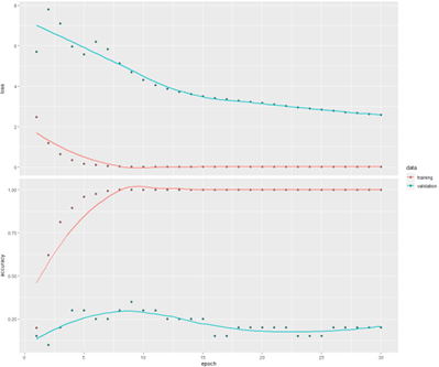
> plot(mlp_fit)

The model is severely overfitted. The accuracy of the training set has reached 1 in the 8th training cycle, and the accuracy of the validation set is only 0.3 at this time, and the accuracy of the validation set in the subsequent training cycles shows a downward trend.
Finally, use predict_classes() to make class predictions on the test set and see the actual and predicted labels for each test sample.

 > pred_label <- mlp_model %>% 
+   predict_classes(x=array_reshape(test_flower_tensors,
+                              c(dim(test_flower_tensors)[1],128*128*3)),
+                   verbose = 0) # 对测试集进行预测
> 
> result <- data.frame(flowers[-index,], # 测试集实际标签
+                 'pred_label' = pred_label) # 测试集预测标签
> result$isright <- ifelse(result$label==result$pred_label,1,0) # 判断预测是否正确
> result  # 查看结果
        file     label   pred_label  isright
10  0010.png     0          0       1
17  0017.png     0          9       0
30  0030.png     6          1       0
35  0035.png     3          5       0
43  0043.png     7          7       1
45  0045.png     1          0       0
52  0052.png     4          8       0
60  0060.png     8          0       0
64  0064.png     8          8       1
70  0070.png     4          8       0
71  0071.png     9          5       0
76  0076.png     3          5       0
95  0095.png     1          1       1
123 0123.png     4          5       0
160 0160.png     3          5       0
162 0162.png     9          7       0
197 0197.png     6          3       0
201 0201.png     1          5       0
207 0207.png     0          0       1

Out of the 19 training samples, only 5 samples have their labels predicted correctly, namely 0010.png, 0043.png, 0064.png, 0095.png, and 0207.png.

The overall accuracy of the test set is 26.3%, which is only 10% better than the baseline (there are 10 categories in total, and there is a 10% chance of guessing right by random guessing). Obviously, the results of this model are not very satisfactory. The next step is to build a simple Convolutional Neural Network (CNN) and see the predictive power of the model.

▌CNN model establishment and prediction

In this case, our convolutional neural network contains only one convolutional layer. The following program code implements model creation, compilation and training.

 > cnn_model %>%
+   layer_conv_2d(filter = 32, kernel_size = c(3,3), input_shape = c(128, 128, 3)) %>%
+   layer_activation("relu") %>%
+   layer_max_pooling_2d(pool_size = c(2,2)) %>% 
+   layer_flatten() %>%
+   layer_dense(64) %>%
+   layer_activation("relu") %>%
+   layer_dropout(0.5) %>%
+   layer_dense(10) %>%
+   layer_activation("softmax")
> 
> cnn_model %>% compile(
+   loss = "categorical_crossentropy",
+   optimizer = optimizer_rmsprop(lr = 0.001, decay = 1e-6),
+   metrics = "accuracy"
+ )
> cnn_fit <- cnn_model %>%
+   fit(
+     x=train_flower_tensors,
+     y=train_flower_targets,
+     shuffle=T,
+     batch_size=64,
+     validation_split=0.1,
+     epochs=30
+   )
> plot(cnn_fit)

The effect of CNN is significantly better than that of MLP. Use the trained CNN model to make predictions on the test set and calculate the overall accuracy of the test set.

 > pred_label1 <- cnn_model %>% 
+   predict_classes(x=test_flower_tensors,
+                verbose = 0) # 对测试集进行预测
> 
> cnn_result <- data.frame(flowers[-index,], # 测试集实际标签
+                     'pred_label' = pred_label1) # 测试集预测标签
> cnn_result$isright <- ifelse(cnn_result$label==cnn_result$pred_label,1,0) #判断预测正确性
> # cnn_result  # 查看结果
> # 查看测试集的整体准确率
> cat(paste('测试集的准确率为:',
+         round(sum(cnn_result$isright)*100/dim(cnn_result)[1],1),"%"))
测试集的准确率为: 57.9 %

The prediction accuracy of the CNN model on the test set reaches 58%, which is much better than the MLP model.
At the end of the book, data augmentation techniques are used to further improve the accuracy of the model. The prediction accuracy of the data augmentation technology model on the test set reached 68%, which is a big improvement.

Microsoft Most Valuable Professional (MVP)

The Microsoft Most Valuable Professional is a global award given to third-party technology professionals by Microsoft Corporation. For 29 years, technology community leaders around the world have received this award for sharing their expertise and experience in technology communities both online and offline.

MVPs are a carefully selected team of experts who represent the most skilled and intelligent minds, passionate and helpful experts who are deeply invested in the community. MVP is committed to helping others and maximizing the use of Microsoft technologies by Microsoft technical community users by speaking, forum Q&A, creating websites, writing blogs, sharing videos, open source projects, organizing conferences, etc.

For more details, please visit the official website: https://mvp.microsoft.com/zh-cn

Long press to identify the QR code and follow Microsoft Developer MSDN

Click to learn more deep learning knowledge ~