Analysis of Nearest Neighbor Search Algorithm​

Introduction

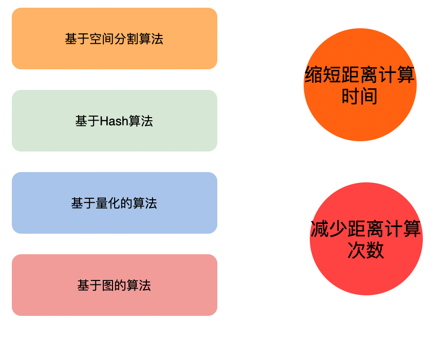
With the development and popularization of deep learning, many unstructured data are represented as high-dimensional vectors and searched by nearest neighbors, which fulfills the retrieval needs of various scenarios, such as face recognition, image search, and product recommendation search. On the other hand, with the development of Internet technology and the popularization of 5G technology, the data generated has exploded. How to complete the search accurately and efficiently in the massive data has become a research hotspot. Various senior experts have proposed different algorithms. Today we Let’s briefly talk about the most common nearest neighbor search algorithms.

main algorithm

Kd-Tree

K-dimension tree, binary tree structure, divides data points in k-dimensional space (such as two-dimensional (x, y), three-dimensional (x, y, z), k-dimensional (x, y, z..)).

Construction process <br>Determine the value of the split domain (polling or maximum variance) Determine the domain value of Node-data (median or average) Determine the left and right subspaces Recursively construct the left and right subspaces

Query process <br>Perform binary search to find leaf nodes Backtrack the search path and enter the subspace of other candidate nodes to query for points with a closer distance Repeat step 2 until the search path is empty

Performance <br>Ideal case complexity is O(K log(N)) Worst case (when the neighborhood of the query point intersects the space on both sides of the split hyperplane, the number of backtracking is greatly increased) When the complexity of the dimension is relatively large, the performance of direct use of Kd tree for fast retrieval (dimension exceeding 20) drops sharply, almost close to linear scan.

improve algorithm
Best-Bin-First: By setting the priority queue (sorting the nodes on the "query path", such as sorting by the distance between the respective split hyperplane and the query point) and running the timeout limit (limiting the searched leaf node tree) to obtain the approximate nearest neighbors, effectively reducing the number of backtracking. After using the BBF query mechanism, the Kd tree can be effectively extended to high-dimensional data sets.

Randomized Kd tree: Improve search performance by building multiple Kd trees in different directions and searching a partial number of nodes in parallel on each Kd tree (mainly solves the problem that the BBF algorithm increases with the increase of Max-search nodes, and the revenue decreases)

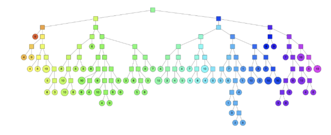
Hierarchical k-means trees

Similar to k-means tree, a binary tree is built by clustering so that the time complexity of searching for each point is O(log n).

Build process:
Randomly select two points, perform clustering with k equal to 2, and divide the dataset into the divided subspaces with a hyperplane perpendicular to the two cluster centers, and recursively and iteratively continue to divide until each subspace has at most only left. K data nodes finally form a binary tree structure. The leaf node records the original data node, and the intermediate node records the information of the split hyperplane

search process

• Start the comparison from the root node, find the leaf node, and record the nodes on the path into the priority queue
• Perform backtracking, pick nodes from the priority queue and re-execute the lookup
• Each lookup records untraversed nodes in the path to the priority queue
• Terminate the search when the number of traversed nodes reaches the specified threshold

performance

• Search performance is not particularly stable, performing well on some datasets and a little worse on others
• It takes a long time to build the tree, which can be optimized by setting the number of iterations of kmeans

LSH

If two points in a high-dimensional space of Locality-Sensitive Hashing are very close, their hash value has a high probability to be the same; if the distance between two points is far, their probability of the same hash value is very small.

Generally, a hash function that satisfies the conditions is selected according to specific needs. (d1,d2,p1,p2)-sensitive satisfies the following two conditions (D is the spatial distance measure, and Pr is the probability):

• If the distance between two points p and q in space D(p,q)<d1, then Pr(h(p)=h(q))>p1
• If the distance between two points p and q in space D(p,q)>d2, then Pr(h(p)=h(q))<p2

Build indexes offline

Choose a hash function that satisfies (𝑅,𝑐𝑅,𝑃1,𝑃2)-sensive; determine the number of hash tables 𝐿 according to the accuracy of the search result (that is, the probability that adjacent data is found), within each table The number of hash functions (that is, the key length of the hash 𝐾), and the parameters related to the LSH hash function itself; use the above hash function group to map all the data in the collection to one or more hash tables , complete the index establishment.

Find it online

Map the query vector 𝑞 through the hash function to obtain the number in the corresponding hash table, and take out the corresponding numbered vectors in all hash tables, (to ensure the search speed, usually only the first 2𝐿 are taken) Linearize these 2𝐿 vectors Find, returning the most similar vector to the query vector.

The query time is mainly:
Calculate the hash value of q (table id) + calculate the distance between q and the midpoint of the table

In terms of query effect, the retrieval accuracy is reduced due to the loss of a large amount of original information.

PQ

Product quantization, decomposes the original vector space into the Cartesian product of several low-dimensional vector spaces, and quantizes the low-dimensional vector spaces obtained by the decomposition, so that each vector can be composed of multiple low-dimensional space. Quantized code combined representation.

The optimal quantization algorithm needs to be selected, and the well-known k-means algorithm is a nearly optimal quantization algorithm.

quantify

The process of quantization using k-means

1. Divide the original vector into m groups, use k-means clustering in each group, and output m groups, each group has multiple cluster centers
2. Encode the original vector as an m-dimensional vector, each element in the vector represents the id of the cluster center of the group in which it belongs

query process

1. Divide the search query into sub-vectors, calculate the distances between the sub-vectors and all cluster centers of the corresponding segment, and get the distance table (m×k*matrix)
2. Traverse the vectors in the sample library, calculate the distance between each sample and the query vector according to the distance table, and return the k samples with the closest distance

distance calculation

SDC (symmetric distance computation), a symmetric distance calculation method, performs PQ quantization on both the query vector and the vectors in the sample library, and at the same time, the distance between each cluster center of each set of vectors will be calculated in the construction phase, and the distance of k*k will be generated. Table, when calculating the query vector and the vector in the sample library in the query stage, just look up the table, which reduces the calculation process, but amplifies the error.

ADC (Asymmetric distance computation), an asymmetric distance calculation scheme, only performs PQ quantization on the vectors in the sample library, calculates the distance between the query vector and m groups of cluster centers in the query stage, generates an m*k distance table, and then checks The distance between the table calculation and the vector in the sample library needs to be calculated in real time for the query vector every time, which increases the calculation overhead, but the error is small.

optimization

IVFPQ, based on the inverted product quantization algorithm, increases the coarse quantization stage, clusters the samples, divides them into smaller regions, and reduces the amount of candidate set data (previously, the full amount of samples needs to be traversed, and the time complexity is O(N* M)).

HNSW

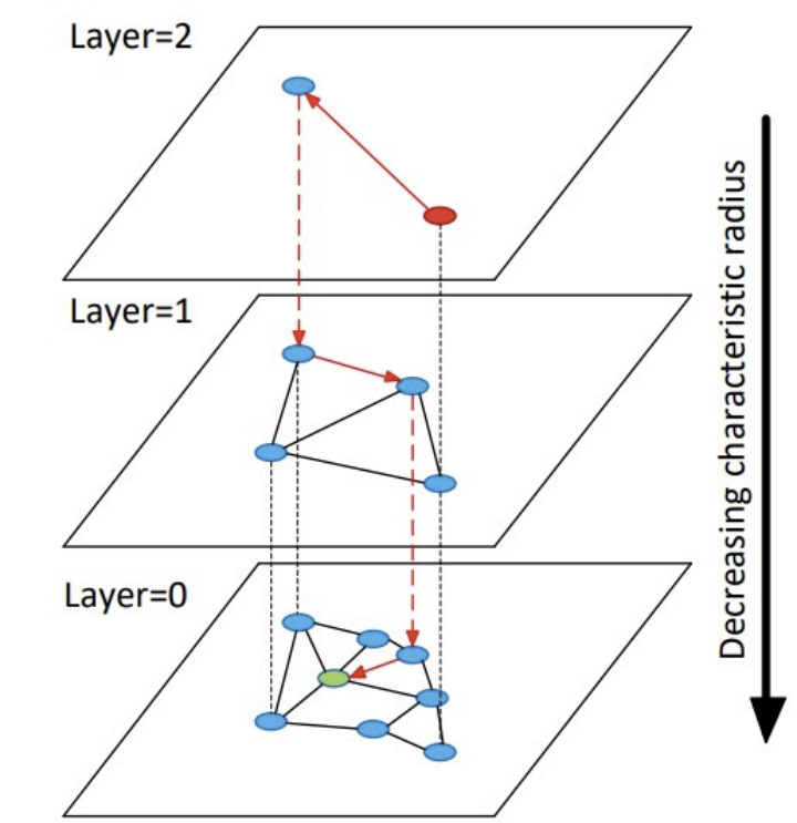
The improved graph-based algorithm based on the NSW algorithm uses a hierarchical structure, and selects the neighbors of a node through heuristic methods at each layer (to ensure global connectivity) to form a connected graph.

Mapping process

1. Calculate the maximum level l of the node;
2. Randomly select the initial entry point ep, and L is the largest layer where the ep point is located;
3. In layers L~l+1, each layer performs operations: find the node ep closest to the node to be inserted in the current layer, and use it as the input of the next layer;
4. Below the l layer is the insertion layer of the element to be inserted, starting from ep to find the ef nodes closest to the element to be inserted, select M nodes to be connected to the node to be inserted, and use these M nodes as the input of the next layer;
5. In layers 1-1 to 0, operations are performed at each layer: start the search from M nodes, find the ef nodes that are closest to the node to be inserted, and select M nodes to connect to the element to be inserted

query process

1. From the top layer to the penultimate layer, perform the operation in a loop: find the node closest to the query node in the current layer and put it into the candidate set, and select the node closest to the query node from the candidate set as the entry point of the next layer;
2. Search the bottom layer from the nearest point obtained from the upper layer, and get ef nearest neighbors and put them into the candidate set;
3. Select topk from the candidate set.

accomplish

At present, there are relatively mature libraries that implement various mainstream neighbor search algorithms. In the project, these basic libraries can be used to build corresponding neighbor search services. Among them, the faiss library is widely used, which is open sourced by Facebook and supports different algorithms. At the same time, it also supports the construction of k-nearest neighbor search on ultra-large-scale datasets and supports GPU to accelerate index construction and query. At the same time, the community is active. Considering performance and maintainability, the faiss library is a better choice for building a nearest neighbor search service.

Summarize

This article shows several common nearest neighbor search algorithms, and briefly analyzes the principles of each algorithm; with the continuous development of deep learning, there are more and more needs for neighbor search in different scenarios, and new algorithms must be continuously developed. Emerging, each algorithm has its own suitable scenarios. When choosing different algorithms, it is necessary to combine the needs of the business, such as the size of the data, the effect of recall, performance, resource consumption and other factors. By understanding the implementation of different algorithms, you can Choose an algorithm that is more suitable for your current business.

*Text/Zhang Lin
@德物科技public account