人工智能 - Deep Learning Tutorial | Network Optimization: Hyperparameter Tuning, Regularization, Batch Normalization, and Program Frameworks - ShowMeAI研究中心

ShowMeAI研究中心

Author: Han Xinzi @ShowMeAI
Tutorial address : https://www.showmeai.tech/tutorials/35
Address of this article : https://www.showmeai.tech/article-detail/218
Disclaimer: All rights reserved, please contact the platform and the author for reprinting and indicate the source
Bookmark ShowMeAI for more exciting content

第2门课改善深层神经网络：超参数调试、正则化以及优化，第3周：超参数调试，batch正则化和程序框架

This series is based on the learning and summary of Mr. Wu Enda's "Deep Learning Specialization". The corresponding course videos can be viewed here .

introduction

In ShowMeAI's previous article, Neural Network Optimization Algorithms , we introduced the following:

batch/mini-batch/ Stochastic gradient descent
Exponentially weighted averages and bias correction
Momentum Gradient Descent, RMSprop and Adam Algorithms
learning rate decay
The concept and conclusion of local optimum

In this article, we will focus on the three parts of hyperparameter debugging, BN (Batch Normalization) and deep learning programming framework.

1. Hyperparameter debugging

调试处理 Tuning Process

There are many hyperparameters ( Hyperparameters ) that need to be debugged for deep neural networks. Let's take a look at how to debug them.

1.1 Ranking of importance

Among the hyperparameters mentioned by Mr. Wu Enda, the order of importance is (for reference only):

超参数调试处理

Most important :

Learning rate$ \alpha$

Next important :

$ \beta$ : Momentum decay parameter, usually set to 0.9
$ n^{[l]}$ : The number of neurons in each hidden layer (#hidden units)
Size of Mini-Batch

Important again :

$ \beta_1$ , $ \beta_2$ , $ \varepsilon$ : Hyperparameters of Adam's optimization algorithm, usually set to 0.9, 0.999, $ 10^{-8}$
$ L$ : the number of neural network layers (#layers)
decay_rate: learning decay rate

1.2 Parameter tuning skills

Let's take a look at the hyperparameter selection and debugging methods of neural networks. In traditional machine learning, we select any number of points equidistantly for each parameter, and then use the parameter combinations corresponding to different points for training, and finally select the best one according to the performance on the validation set. parameter.

For example, there are two parameters to be debugged, Hyperparameter 1 and Hyperparameter 2. On each parameter, select $ 5$ points at even intervals, thus forming $ 5 \times 5=25$ parameter combinations, as shown in the figure shown. This approach works better when there are fewer parameters.

超参数调试处理

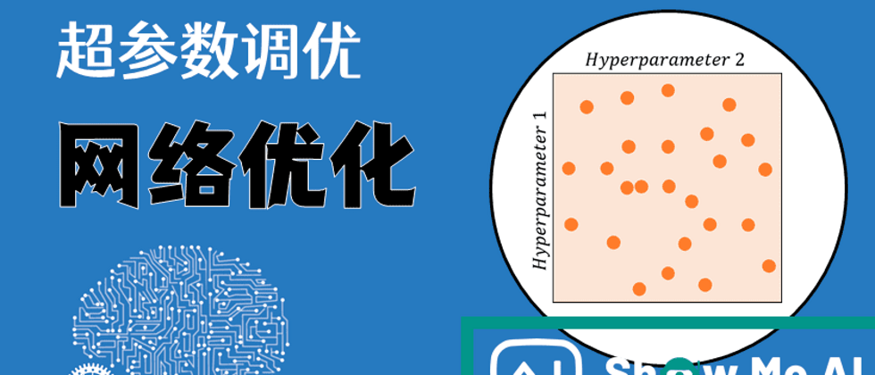
However, in the deep neural network model, we generally do not use this method of evenly spaced points, and a better way is to use random selection. That is to say, for the above example, we randomly select 25 points as hyperparameters to be debugged, as shown in the following figure:

超参数调试处理

The purpose of randomizing the selection of parameters is to obtain as many parameter combinations as possible. Still in the above example, with uniform sampling, there are only 5 cases for each parameter; with random sampling, there are 25 possible cases for each parameter, so it is more likely to get the best parameter combination.

Another benefit of this approach is that the selection between parameters of different importance is better . Assuming that hyperparameter1 is $ \alpha$ and hyperparameter2 is $ \varepsilon$, obviously the importance of the two is different.

If the first method of uniform sampling is used, the effect of $ \varepsilon$ is small, equivalent to only 5 $ \alpha$ values being selected.
If the second method of random sampling is used, both $ \varepsilon$ and $ \alpha$ have the potential to choose 25 different values. This greatly increases the number of $ \alpha$ debugs, making it more likely to select the optimal value.

In fact, in practical applications, when it is completely unknown which parameter is more important, random sampling can effectively solve this problem, but uniform sampling cannot do this.

超参数调试处理

After random sampling, we may get some regional models that perform better. However, in order to get more precise optimal parameters , we should continue to do a coarse to fine sampling scheme on the selected regions. That is, zoom in on the area with better performance, and then do more dense random sampling of this area. For example, do another 25 random sampling of the square area in the lower right corner of the figure to get the best parameters.

In summary, the skills of the hyperparameter debugging process are summarized as follows:

① Randomly select points (rather than uniformly), and use these points to experiment with the effect of hyperparameters . The reason for this is that it is difficult to know in advance how important the hyperparameters are, and more experiments can be done by choosing more values;
②From rough to fine : a small area composed of points with good focusing effect, in which values are more densely taken, and so on;

1.3 Choose the right range

为超参数选择和适合范围 Using An Appropriate Scale to Pick Hyperparameters

The previous paragraph talked about using random sampling to debug hyperparameters. For some hyperparameters, uniform scale sampling is possible, but for some hyperparameters, different appropriate scales need to be selected for random sampling. for example:

① For hyperparameters (#layers) and (#hidden units) , both are positive integers, which can be uniformly sampled randomly, that is, the scale of each change of hyperparameters is consistent (for example, each change is 1, like a scale Like a ruler, the scale is even).

② For the hyperparameter $ \alpha$ , the range to be adjusted is $ [0.0001, 1]$ .

If uniform random sampling is used, then 90% of the sampling points are distributed between $ [0.1, 1]$ and only 10% are distributed between $ [0.0001, 0.1]$. This is not very good in practice, because the optimal $ \alpha$ value may be mainly distributed between $ [0.0001, 0.1]$ and $ [0.1, 1]$ $ \alpha$ values don't work well.
We are more concerned with the interval $ [0.0001, 0.1]$ , within which more ticks should be subdivided.

超参数调试处理

For non-uniform sampling, a common practice is to convert linear scale to log scale , convert uniform scale to non-uniform scale , and then perform uniform sampling under log scale. In this way, $ [0.0001, 0.001]$ , $ [0.001, 0.01]$ , $ [0.01, 0.1]$ , $ [0.1, 1]$ Hyperparameters randomly sampled in each interval The numbers are basically the same, which expands the number of sampled values in the previous $ [0.0001, 0.1]$ interval.

Let's take the important parameters learning rate and momentum decay parameters as an example:

For the learning rate$ \alpha$, it is more reasonable to use a log scale instead of a linear axis: 0.0001, 0.001, 0.01, 0.1, etc., and then randomly and uniformly take values between these scales;
For the momentum decay parameter $ \beta$ , taking 0.9 is equivalent to averaging over 10 values, and taking 0.999 is equivalent to averaging over 1000 values. Consider giving a value to $ 1-\beta$, which is similar to taking the learning rate.

The reason for the above operation is that when $ \beta$ is close to 1, even a small change in $ \beta$ results in a large change in the sensitivity of the result. For example, increasing $ \beta$ from 0.9 to 0.9005 has little effect on the result $ (1/(1-\beta$ )), while $ \beta$ from 0.999 to 0.9995 has a huge effect on the result ( from 1000 values to 2000 values).

1.4 Some suggestions

超参数训练的实践：pandas vs Caviar Hyperparameters Tuning in Practice: Pandas vs Caviar

(1) Deep learning has been applied to many different fields today. Different applications appear to be intermingled, and the hyperparameter settings of one application domain may be common to another domain. People in different application fields should also read more papers in other research fields to find inspiration across fields.

(2) Considering data changes or server changes, it is recommended to re-test or evaluate hyperparameters at least once every few months to obtain the best real-time model;

(3) Decide how you train the model based on the computing resources you have:

超参数调试处理

Panda (Panda Way) : There is a large amount of data in online advertising settings or in the field of computer vision applications, but limited by computing power, it is difficult to test a large number of models at the same time. This can be done in this way: try out a model or a small batch, initialize it, try to get it working, watch it perform, keep tweaking the parameters;
Caviar (caviar method) : have enough computers to test many models in parallel, try many different hyperparameters, and select the model with the best effect;

2.Batch Normalization

Two scholars, Sergey Ioffe and Christian Szegedy, proposed the Batch Normalization (often abbreviated as BN) method in their paper. Batch Normalization not only makes debugging hyperparameters easier, but also makes neural network models more "robust". That is to say, the acceptable range of hyperparameters for better models is larger and more inclusive, making it easier to train a deep neural network.

Next, let's introduce what Batch Normalization is and how it works .

Previously, we used normalization on the input feature $ X$. We can also use the same idea to process the activation value of the hidden layer $ a^{[l]}$ to speed up $ W^{[l+1]}$ and $ b^{[l+1 ]}$ training. In practice, the normalized hidden layer input $ Z^{[l]}$ is often chosen, and here we do the following for the $ l$ hidden layer:

批标准化 Batch Normalization

Among them, $ m$ is the number of samples contained in a single Mini-Batch, and $ \varepsilon$ is to prevent the denominator from being zero, usually $ 10^{-8}$ .

Let's make a visual and detailed explanation of the above BN link from the " sample " and " channel " dimensions. For the input of a certain layer $ N \times D$, the calculation process of our above operation is shown in the figure below. (Note that $ i$ is the sample dimension and $ j$ is the channel dimension)

批标准化 Batch Normalization

The data distribution before and after the above processing is shown in the figure below, we can see the "Normalization" effect of this processing on the data.

批标准化 Batch Normalization

In this way, we make all inputs $ z^{(i)}$ mean 0 and variance 1. But we don't want to rudely make the processed hidden layer unit directly change to mean 0 and variance 1, so that the originally learned data distribution is directly erased. Therefore, we introduce the learnable parameters $ \gamma$ and $ \beta$ to linearly transform $ z_{norm}^{(i)}$ as follows:

批标准化 Batch Normalization

Among them, $ \gamma$ and $ \beta$ are the learning parameters of the model, so various gradient descent algorithms can be used to update the values of $ \gamma$ and $ \beta$, just like updating Neural network weights are the same.

Through reasonable settings of $ \gamma$ and $ \beta$, the mean and variance of $ \tilde z^{(i)}$ can be arbitrary. In this way, we normalize the $ z^{(i)}$ of the hidden layer and replace $ z^{(i)}$ with the resulting $ \tilde z^{(i)}$ .

The learnable parameters $ \gamma$ and $ \beta$ are set in the formula. The reason is that if the input mean of each hidden layer is in the region close to 0, that is, in the linear region of the activation function, it is not conducive to training nonlinear neural networks. , resulting in a less effective model. Therefore, the normalized results need to be further processed with $ \gamma$ and $ \beta$.

2.1 Applying BN to Neural Networks

将 Batch Norm 拟合进神经网络 Fitting Batch Norm into a Neural Network

The above explains the method of BN batch normalization for all neurons in a single hidden layer. The summary diagram is as follows:

批标准化 Batch Normalization

Next, we will study how to apply Bath Norm to the entire neural network. For the L-layer neural network, after the role of Batch Normalization, the overall process is as follows:

批标准化 Batch Normalization

In fact, Batch Normalization is often used on Mini-Batch, which is where its name comes from.

When using Batch Normalization, because the normalization process includes a step of subtracting the mean, $ b$ does not actually play a role, and its numerical effect is implemented by $ \beta$. Therefore, in Batch Normalization, $ b$ can be omitted or temporarily set to 0.

When using the gradient descent algorithm, iteratively update $ W^{[l]}$ , $ \beta^{[l]}$ and $ \gamma ^{[l]}$ respectively.

In addition to the traditional gradient descent algorithm, optimization algorithms such as momentum gradient descent, RMSProp or Adam mentioned in the neural network optimization algorithm mentioned in the previous article of ShowMeAI can also be used.

2.2 Reasons why BN is effective

为什么batch Norm奏效？ Why Does Batch Norm Work?

There are two reasons why Batch Normalization works well:

By doing similar normalization processing to the input of each neuron in the hidden layer, the training speed of the neural network is improved;
It can reduce the influence of the weight change of the previous layer on the later layer, and the overall network is more robust.

Regarding the second point, if the data distribution of the actual application sample and the training sample is different (the black cat picture and the orange cat picture in the figure below), we say that " Covariate Shift " occurs. In this case, the model is generally retrained. The role of Batch Normalization is to reduce the impact of Covariate Shift, making the model more robust and robust .

批标准化 Batch Normalization

Even if the input value changes, due to the effect of Batch Normalization, the mean and variance remain unchanged (determined by $ \gamma$ and $ \beta$), limiting the parameter update in the previous layer to the value distribution. The degree of influence, so the learning of the later layers becomes easier. Batch Normalization reduces the coupling between $ W$ and $ b$ of each layer, makes each layer more independent, and achieves the effect of self-training and learning.

In addition, Batch Normalization also has a weak regularization effect. Because the mean and variance are calculated on each Mini-Batch rather than the entire dataset, the mean and variance estimated from only this small subset of data will have some noise, so the final calculated $ \tilde z^{( i)}$ also has some noise. Similar to Dropout, this noise prevents neurons from being particularly dependent on any one input feature.

Because Batch Normalization has only a weak regularization effect, it can be used with Dropout for a stronger regularization effect. Noise can be reduced by applying a larger Mini-Batch size, reducing this regularization effect.

Teacher Wu Enda also reminded everyone not to use Batch Normalization as a means of regularization, but as a way to accelerate learning. Regularization is just an undesired side effect, Batch Normalization solves the gradient problem (gradient disappearance and explosion) during backpropagation.

2.3 Batch Normalization in the testing phase

测试时的 Batch Norm Batch Norm at Test Time

Batch Normalization processes the data one by one in the form of Mini-Batch, but during testing, it may be necessary to process each sample one by one, so that $ \mu$ and $ \sigma^2$ cannot be obtained.

In theory, we can put all the training sets into the final neural network model, and then calculate the $ \mu^{[l]}$ and $ \sigma^{2[l] calculated by each hidden layer }$ are used directly as $ \mu$ and $ \sigma$ of the test procedure. However, this method is generally not used in practical applications, but the previously learned exponentially weighted average method is used to predict the $ \mu$ and $ \sigma^2$ of a single sample during the testing process.

测试阶段的BN操作

For the $ l$th hidden layer, consider all Mini-Batch $ \mu^{[l]}$ and $ \sigma^{2[l]}$ under this hidden layer, then Use the exponentially weighted average method to predict the $ \mu^{[l]}$ and $ \sigma^{2[l]}$ of the current single sample. This achieves mean and variance estimates for a single sample of the testing process.

3. Softmax regression

Softmax回归 Softmax Regression

So far, the classification examples introduced are all binary classification problems: there is only one neuron in the output layer of the neural network, indicating the probability that the predicted output$ \hat{y}$ is a positive class$ P(y = 1 \mid x)\ ), \( \hat{y}> 0.5$ is judged as a positive class, otherwise it is judged as a negative class.

For multi-classification problems , use $ C$ to represent the number of categories, then the output layer of the neural network, that is, the number of units in the $ L$ layer$ n^{[L]} = C$ . The output of each neuron in turn corresponds to the probability of belonging to that class, ie $ P(y=c \mid x), c=0,1,...,C-1$ . There is a general form of logistic regression, called Softmax regression , that can handle multi-classification problems.

For the output layer of the Softmax regression model, that is, the $ L$ layer, there are: $ Z^{[L]} = W^{[L]}a^{[L-1]} + b^{[ L]}$

for i in range(L) , with: $ a^{[L]}_i = \frac{e^{Z^{[L]}_i}}{\sum^C_{i=1}e^{ Z^{[L]}_i}}$

is the output of each neuron in the output layer, corresponding to the probability of belonging to this class, satisfying: $ \sum^C_{i=1}a^{[L]}_i = 1$

训练一个 Softmax 分类器 Training a Softmax Classifier

An intuitive calculation example is as follows:

Softmax 回归

The following figure shows the classification boundaries obtained by some softmax linear classifiers

Softmax 回归

3.1 Loss function and cost function

Let's take a look at the loss function of the softmax classifier, which is defined here as: $ L(\hat y, y) = -\sum^C_{j=1}y_jlog\hat y_j$

When $ i$ is the real category of the sample, there are: $ y_j = 0, j \ne i$

Therefore, the loss function can be simplified to: $ L(\hat y, y) = -y_ilog\hat y_i = log \hat y_i$

The cost function for all $ m$ samples is: $ J = \frac{1}{m}\sum^m_{i=1}L(\hat y, y)$

3.2 Gradient descent method

There is only a little difference between the multi-class Softmax regression model and the two-class Logistic regression model in the output layer. After a different derivation process, there are still

$$ dZ^{[L]} = A^{[L]} - Y $$

The other steps of the backpropagation process are also the same as those of logistic regression.

Reference: Softmax Regression - Ufldl

4. Deep Learning Framework

深度学习框架 Deep Learning Frameworks

4.1 More famous frameworks

深度学习框架

Caffe / Caffe2
CNTK
DL4J
Keras
Lasagne
mxnet
PaddlePaddle
TensorFlow
pytorch

4.2 Criteria for choosing a framework

Ease of programming: including the development and iteration of neural networks, and configuring products;
Running speed: especially when training large datasets;
Whether it is truly open: Not only need to be open source, but also need to be well-managed, able to continue to open all functions.

5. Tensorflow

TensorFlow

One of the hottest deep learning frameworks right now is Tensorflow from google. A brief introduction is given below. (For more TensorFlow practical methods, please refer to)

The gradient descent algorithm can be called directly in the Tensorflow framework, which greatly reduces the workload of programmers. For example the following code:

深度学习框架

 import numpy as np
import tensorflow as tf

cofficients = np.array([[1.],[-10.],[25.]])

w = tf.Variable(0,dtype=tf.float32)
x = tf.placeholder(tf.float32,[3,1])
# Tensorflow 重载了加减乘除符号
cost = x[0][0]*w**2 + x[1][0]*w + x[2][0]
# 改变下面这行代码，可以换用更好的优化算法
train = tf.train.GradientDescentOptimizer(0.01).minimize(cost)

init = tf.global_variables_initializer()
session = tf.Session()
session.run(init)
for i in range(1000):
    session.run(train, feed_dict=(x:coefficients))
print(session.run(w))

The print is 4.99999, which is basically the result we need. Changing the value of cofficients can give different results w.
In the above code:

 session = tf.Session()
session.run(init)
print(session.run(w))

It is also possible to write:

 with tf.Session() as session:
    session.run(init)
    print(session.run(w))

The with statement is suitable for accessing resources, ensuring that necessary "cleanup" operations are performed regardless of whether an exception occurs during use, and resources are released, such as automatic closing of files after use, automatic acquisition and release of locks in threads, etc.

To learn more about Tensorflow, please refer to the official documentation .

References:

Featured Recommendations in ShowMeAI Series Tutorials

ShowMeAI用知识加速每一次技术成长

Deep Learning Tutorial | Network Optimization: Hyperparameter Tuning, Regularization, Batch Normalization, and Program Frameworks

introduction

1. Hyperparameter debugging

1.1 Ranking of importance

Most important :

Next important :

Important again :

1.2 Parameter tuning skills

1.3 Choose the right range

1.4 Some suggestions

2.Batch Normalization

2.1 Applying BN to Neural Networks

2.2 Reasons why BN is effective

2.3 Batch Normalization in the testing phase

3. Softmax regression

3.1 Loss function and cost function

3.2 Gradient descent method

4. Deep Learning Framework

4.1 More famous frameworks

4.2 Criteria for choosing a framework

5. Tensorflow

References:

recommended article

Featured Recommendations in ShowMeAI Series Tutorials

用户bPcV4sA

引用和评论

数据分析大作战，SQL V.S. Python，来看看这些考题你都会吗 ⛵

从云计算一哥到全球生成式 AI 前行者：回顾 re:Invent 2024 三项重要发布

【AI日志分析】基于机器学习的异常检测：告别传统规则的智能进阶

从 re:Invent 2024 看 AWS 最前沿的 AI 基础设施架构

智能图像识别系统设计与实现

合合信息在视觉内容安全领域的创新与应用-应对伪造挑战的前沿进展

从 DeepSeek 看25年前端的一个小趋势